The 7 essential functions at a glance:
- SUM — Adds a range of values: =SUM(A1:A10)
- AVERAGE — Returns the mean of a range: =AVERAGE(B1:B10)
- COUNT — Counts numeric cells: =COUNT(A1:A20)
- MIN — Returns the smallest value: =MIN(C1:C15)
- MAX — Returns the largest value: =MAX(C1:C15)
- IF — Tests a condition and returns one of two values: =IF(A1>100,"High","Low")
- XLOOKUP — Searches a range and returns a match: =XLOOKUP(A2,D2:D100,E2:E100)
How this reference is organized:
- Math & Arithmetic
- Text
- Logical
- Lookup & Reference
- Date & Time
- Statistical
- Financial
How to use this guide: treat it as a syntax reference, not a memorization list. When you know the function you need but can't recall the argument order, come back here. Active practice is what builds real speed.
Quick keyboard shortcuts for entering functions:
- = — Start any formula
- Ctrl + Shift + Enter — Enter an array formula (legacy Excel)
- Tab — Accept an autocomplete suggestion
- Shift + F3 — Open the Insert Function dialog
- Ctrl + ` — Toggle formula view to see all formulas at once
*
Excel functions by category: your complete formula reference
Excel includes over 400 built-in functions, and the most practical way to learn them is by category rather than trying to memorize an alphabetical list. Each category below includes the functions you'll actually use, with syntax and a quick example of when to reach for them.
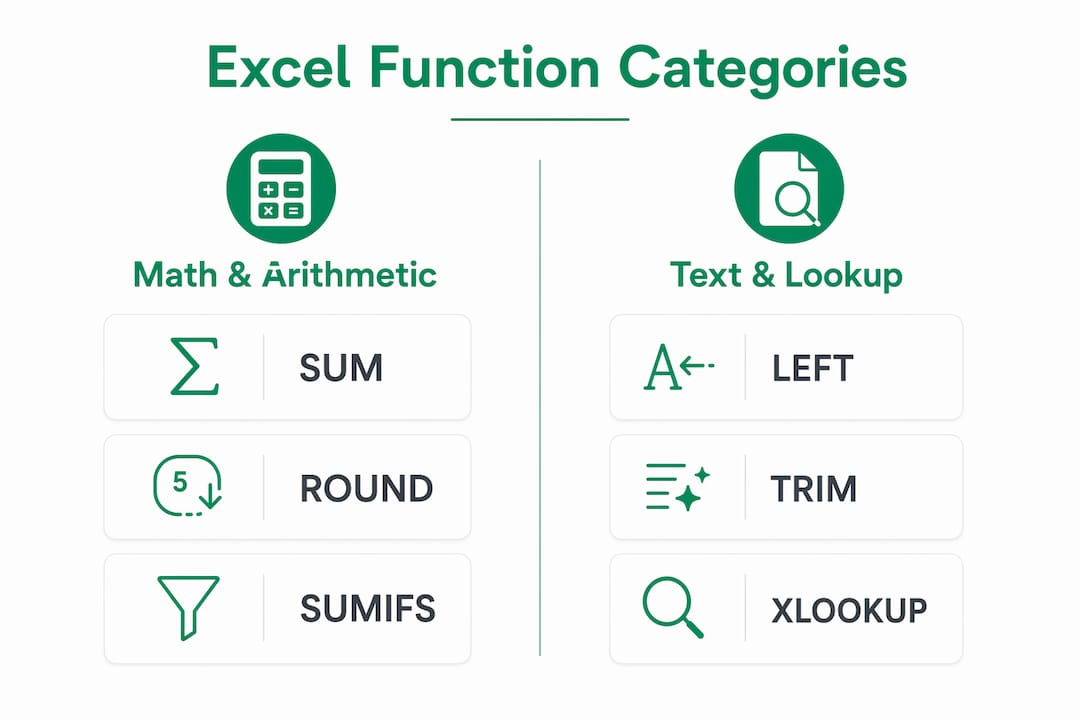
Math & arithmetic functions
These handle number crunching, rounding, and conditional summing. They're the backbone of any financial or data model.

| Function | Syntax | What it does |
| SUM | =SUM(A1:A10) | Adds all values in a range |
| SUMIF | =SUMIF(range,criteria,sum_range) | Adds values that meet one condition |
| SUMIFS | =SUMIFS(sum_range,range1,crit1,range2,crit2) | Adds values meeting multiple conditions |
| ROUND | =ROUND(A1,2) | Rounds to a specified number of digits |
| INT | =INT(A1) | Rounds down to the nearest integer |
| MOD | =MOD(A1,B1) | Returns the remainder after division |
| ABS | =ABS(A1) | Returns the absolute (positive) value |
Pro Tip: Use SUMIFS instead of nesting multiple IF statements around SUM. It's cleaner, faster to write, and far easier to audit later.
Combining ROUND with SUMIFS is a common pattern in financial reporting: =ROUND(SUMIFS(C2:C100,A2:A100,"Q1"),2) gives you a rounded quarterly total in one formula.
Text functions
Text functions clean, extract, and reformat string data. If you've ever imported data from another system and gotten inconsistent capitalization or trailing spaces, these are your first stop.

| Function | Syntax | What it does |
| LEFT | =LEFT(A1,n) | Extracts characters from the left |
| RIGHT | =RIGHT(A1,n) | Extracts characters from the right |
| MID | =MID(A1,3,6) | Extracts from a specific position |
| LEN | =LEN(A1) | Returns the number of characters |
| TRIM | =TRIM(A1) | Removes extra spaces |
| UPPER / LOWER | =UPPER(A1) | Changes case |
| CONCAT | =CONCAT(A1," ",B1) | Joins text from multiple cells |
| TEXTJOIN | =TEXTJOIN(", ",TRUE,A1:A5) | Joins with a delimiter, ignoring blanks |
TRIM is particularly useful before running VLOOKUP or XLOOKUP. A trailing space in a lookup value is invisible but will cause a mismatch every time.
Logical functions
Logical functions let you build decision trees inside a cell. IF is the entry point, but the real power comes when you combine it with AND, OR, and IFS.
- IF: =IF(A1>50,"Pass","Fail") — Returns one value when true, another when false
- AND: =AND(A1>0,B1<100) — Returns TRUE only when all conditions are met
- OR: =OR(A1="Yes",B1="Yes") — Returns TRUE when at least one condition is met
- IFS: =IFS(A1>=90,"A",A1>=80,"B",A1>=70,"C") — Tests multiple conditions in sequence
- IFERROR: =IFERROR(VLOOKUP(A1,D:E,2,0),"Not found") — Returns a custom value when a formula error
- NOT: =NOT(A1="Closed") — Reverses a logical result
Wrapping any lookup in IFERROR is standard practice. Without it, a single missing value turns your clean report into a grid of #N/A errors.
Lookup & reference functions
These functions retrieve data from tables. VLOOKUP dominated for years, but XLOOKUP is now the recommended standard because it defaults to exact matching, works in both directions, and handles errors more gracefully.
| Function | Syntax | Key advantage |
| XLOOKUP | =XLOOKUP(lookup,search_array,return_array,"Not found") | Exact match default, bidirectional |
| VLOOKUP | =VLOOKUP(A1,D:F,2,FALSE) | Legacy; column must be to the right |
| HLOOKUP | =HLOOKUP(A1,lookup_range,row_index,FALSE) | Searches horizontally across rows |
| INDEX | =INDEX(range,row_num) | Returns a value at a specific position |
| MATCH | =MATCH(A1,D1:D100,0) | Returns the position of a value in a range |
| CHOOSE | =CHOOSE(2,"Jan","Feb","Mar") | Returns a value from a list by index |
INDEX + MATCH is still worth knowing. The combination
=INDEX(B1:B100,MATCH(A1,D1:D100,0)) replicates XLOOKUP behavior and works in older Excel versions.
Date & time functions
Date functions are indispensable for project tracking, payroll, and any report that needs to calculate elapsed time or extract parts of a date.
- TODAY: =TODAY() — Returns today's date, updates automatically
- NOW: =NOW() — Returns the current date and time
- DATE: =DATE(2026,3,15) — Constructs a date from year, month, day
- DATEDIF: =DATEDIF(A1,B1,"D") — Calculates the difference between two dates in days, months, or years
- EOMONTH: =EOMONTH(A1,0) — Returns the last day of the month
- WEEKDAY: =WEEKDAY(A1,2) — Returns the day of the week as a number
- NETWORKDAYS: =NETWORKDAYS(A1,B1) — Counts working days between two dates, excluding weekends
NETWORKDAYS is a hidden gem for project managers. Add a holiday range as the third argument and it automatically skips those days too:
=NETWORKDAYS(A1,B1,H1:H10).
Statistical functions
Statistical functions go beyond simple averages to give you distributions, rankings, and conditional counts.
| Function | Syntax | What it does |
| AVERAGE | =AVERAGE(A1:A50) | Arithmetic mean |
| MEDIAN | =MEDIAN(A1:A50) | Middle value in a sorted set |
| MODE.SNGL | =MODE.SNGL(A1:A50) | Most frequently occurring value |
| STDEV.S | =STDEV.S(A1:A50) | Standard deviation for a sample |
| COUNTIF | =COUNTIF(A1:A50,">100") | Counts cells meeting one condition |
| COUNTIFS | =COUNTIFS(A1:A50,">100",B1:B50,"Active") | Counts cells meeting multiple conditions |
| RANK.EQ | =RANK.EQ(number,ref,order) | Ranks a value within a range |
| LARGE / SMALL | =LARGE(range,k) | Returns the nth largest or smallest value |
MEDIAN often tells a more honest story than AVERAGE when your data has outliers. A salary dataset with a few executives at the top will skew the average significantly, while the median stays grounded.
Financial functions
These are the core functions for loan analysis, investment valuation, and depreciation calculations. Finance teams use them constantly; analysts preparing for Excel certification exams need them cold.
- PMT: =PMT(rate,nper,pv) — Calculates the periodic payment for a loan
- PV: =PV(rate,nper,pmt) — Returns the present value of an investment
- FV: =FV(rate,nper,pmt,pv) — Returns the future value of an investment
- NPV: =NPV(rate,value1,value2,...) — Calculates net present value of cash flows
- IRR: =IRR(values) — Returns the internal rate of return for a series of cash flows
- RATE: =RATE(nper,pmt,pv) — Calculates the interest rate per period
- SLN: =SLN(cost,salvage,life) — Straight-line depreciation per period
For PMT, remember that the rate must match the period. A 6% annual rate on a monthly loan becomes
0.06/12 in the formula:
=PMT(0.06/12,60,-20000).
Combining functions: nested formula patterns
The real power in Excel comes from nesting. A few patterns that show up constantly in professional spreadsheets:
- IFERROR + XLOOKUP: =IFERROR(XLOOKUP(A2,D:D,E:E),"Missing") — Clean lookup with a fallback
- IF + AND: =IF(AND(A1>0,B1="Active"),"Eligible","Not eligible") — Multi-condition decision
- SUMIFS + DATE: =SUMIFS(C:C,A:A,">="&DATE(2026,1,1),A:A,"<="&DATE(2026,3,31)) — Sum by date range
- TEXT + CONCAT: =CONCAT(LEFT(A1,3),"-",TEXT(B1,"000")) — Build formatted codes from parts
- INDEX + MATCH: =INDEX(B:B,MATCH(1,(A:A=D1)*(C:C=E1),0)) — Two-condition lookup (Ctrl+Shift+Enter in legacy Excel)
*
Common Excel errors and how to fix them
Every Excel user hits these errors. The good news is that each one points directly at its own cause, so diagnosis is usually fast once you know the pattern. Understanding what triggers each error is the fastest path to cleaner, more reliable spreadsheets.
#N/A — Value not found
- Cause: A lookup function can't find the search value in the specified range.
- Fix: Check for trailing spaces with TRIM, verify the lookup column is the first column in VLOOKUP, or switch to XLOOKUP which handles mismatches more gracefully.
- Prevention: Wrap the lookup in IFERROR: =IFERROR(XLOOKUP(A1,D:D,E:E),"Not found")
#VALUE! — Wrong data type
- Cause: A formula expects a number but receives text, or vice versa.
- Fix: Use ISNUMBER or ISTEXT to check cell types. Convert text-formatted numbers with VALUE(): =VALUE(A1).
- Prevention: Validate data entry with Data Validation rules before formulas run on the input.
#REF! — Invalid cell reference
- Cause: A formula references a cell that no longer exists, usually because a row or column was deleted.
- Fix: Re-enter the formula with the correct reference. Use named ranges to make references deletion-proof.
- Prevention: Name your key ranges (Formulas tab > Name Manager) so deleting a row doesn't silently break a formula elsewhere.
#DIV/0! — Division by zero
- Cause: A formula divides by a cell that is empty or contains zero.
- Fix: =IF(B1=0,"N/A",A1/B1) or =IFERROR(A1/B1,"N/A")
- Prevention: Always check whether a denominator can realistically be zero before building the formula.
#NAME? — Unrecognized formula name
- Cause: Excel doesn't recognize the function name, usually due to a typo or a missing add-in.
- Fix: Check spelling. If the function is real and spelled correctly, verify it's available in your Excel version (some Excel 365 functions don't exist in Excel 2019).
- Prevention: Use the formula autocomplete dropdown rather than typing function names from scratch.
#NUM! — Invalid numeric value
- Cause: A formula produces a number too large or too small for Excel to display, or an argument is mathematically impossible (like taking the square root of a negative number).
- Fix: Check the input values feeding the formula. For IRR, make sure the cash flow series includes at least one positive and one negative value.
Using Formula Auditing tools to debug formulas
The Formula Auditing toolbar (Formulas tab > Formula Auditing) is one of the most underused features in Excel. Trace Precedents shows you which cells feed into a formula with blue arrows, and Trace Dependents shows which cells rely on the selected cell. When a formula produces a wrong result but no error code, Evaluate Formula (also in that toolbar) steps through the calculation one argument at a time, which is often the fastest way to find where the logic breaks.
Pro Tip: Press F2 on any cell containing a formula to enter edit mode. Excel color-codes each referenced range, making it immediately obvious if a range is off by a row or column.
*
New Excel 365 functions you should be using in 2026
The shift to dynamic array functions in Excel 365 changed how spreadsheets are built. These functions spill results automatically into adjacent cells, eliminating the need for helper columns and repetitive formulas copied down a range.
The five functions that matter most:
- FILTER: =FILTER(A2:C100,B2:B100="West") — Returns only the rows that meet your criteria, spilling results dynamically
- UNIQUE: =UNIQUE(A2:A100) — Extracts a deduplicated list from a column, updating automatically when source data changes
- SORT: =SORT(A2:B50,2,-1) — Sorts a range by a specified column, ascending or descending
- SEQUENCE: =SEQUENCE(10,1,1,1) — Generates a series of numbers (rows, columns, start, step)
- XLOOKUP: =XLOOKUP(A2,D2:D100,E2:E100,"Not found",0) — The modern replacement for VLOOKUP, with exact match as the default
XLOOKUP vs. VLOOKUP: what actually changed
| Feature | VLOOKUP | XLOOKUP |
| Default match type | Approximate | Exact |
| Lookup direction | Left column only | Any column, any direction |
| Return multiple columns | No | Yes |
| Error handling built in | No | Yes (4th argument) |
| Works in Excel 2019 | Yes | No (Excel 365 only) |
VLOOKUP's biggest trap is its default approximate match behavior. If you forget to add FALSE as the fourth argument, it can return a plausible-looking wrong answer with no error message. XLOOKUP defaults to exact matching, so that class of silent error disappears.
Practical scenarios where dynamic arrays save real time:
- Building a unique customer list from a transaction log: =UNIQUE(B2:B5000) replaces a manual Remove Duplicates step that you'd have to repeat every time data updates.
- Creating a filtered report for a specific region without a pivot table: =FILTER(A2:D500,C2:C500="Northeast") updates the moment the source data changes.
- Generating a numbered list for a dropdown or template: =SEQUENCE(12,1,1,1) produces 1 through 12 instantly.
Dynamic arrays also work together.
=SORT(UNIQUE(B2:B500)) returns a sorted, deduplicated list in a single formula. That combination used to require a pivot table or a VBA macro.
*
How to actually get good at Excel functions
The most common mistake people make when learning Excel is treating a formula reference as a study guide. Cheat sheets work best as syntax references, not memorization tools. You use them when you know the function you need but can't remember whether XLOOKUP's return array comes before or after the search array. The goal is to understand the logic, then use the reference to fill in the details.
Understanding formula logic means knowing why a function works, not just what it returns. When you understand that MATCH returns a position number and INDEX uses that position to retrieve a value, you can build INDEX+MATCH from first principles. When you only memorize the syntax, a single unfamiliar argument throws you off completely.
Active practice builds the muscle memory that passive reading never does. Typing a formula, getting it wrong, seeing the error, and fixing it is what actually makes the syntax stick. Reading about SUMIFS is not the same as writing one against a real dataset and watching it return the wrong number because you put the sum range last instead of first.
One of the best ways to build that practice habit is through Logicexcel's free interactive exercises, which put you inside a real Excel-like environment with instant feedback. There's no software to install and no account required. The platform covers everything from basic SUM and COUNT exercises to more advanced formula combinations, and the feedback loop is immediate enough that you correct mistakes before they become habits.
Pro Tip: Work with your own real data whenever possible. Import a dataset from your actual job or a public source like data.gov, then practice writing formulas against it. The context makes the logic stick far faster than abstract exercises.
The golden rule of Excel formula writing is to never hardcode numbers inside a formula. Write =A1B1 instead of =A11.08. When the tax rate changes, you update one cell rather than hunting through fifty formulas. This single habit prevents more errors than any other practice.
For structured learning that goes beyond a single cheat sheet, Logicexcel's Excel learning guides cover formulas, functions, shortcuts, and skills in a step-by-step format built for people who want to move from reference-dependent to genuinely fluent. If you're preparing for a certification like the MO-200 or MO-201, the platform also offers targeted assessment prep so you're practicing the exact skills the test covers.
 *
*
Key Takeaways
The most efficient path to Excel fluency is learning function categories first, practicing with real data, and using a cheat sheet only to recall syntax you already understand.
| Point | Details |
| Start with 7 core functions | SUM, AVERAGE, COUNT, MIN, MAX, IF, and XLOOKUP cover most daily spreadsheet tasks. |
| Learn by category | Excel has over 400 functions; organizing them by type (Math, Text, Logical, Lookup, Date, Statistical, Financial) makes them learnable. |
| Errors point at their cause | Each error code (#N/A, #VALUE!, #REF!, #DIV/0!, #NAME?) has a specific trigger; recognizing the pattern speeds up fixes. |
| Adopt Excel 365 dynamic arrays | FILTER, UNIQUE, SORT, and XLOOKUP eliminate helper columns and reduce formula complexity. |
| Never hardcode values in formulas | Referencing cells instead of typing numbers directly keeps spreadsheets accurate and easy to update. |
*
FAQ
What are the 7 basic Excel formulas?
The seven foundational Excel formulas are SUM, AVERAGE, COUNT, MIN, MAX, IF, and XLOOKUP. These cover arithmetic, conditional logic, and data retrieval for most everyday spreadsheet tasks.
What are the 10 most commonly used Excel functions?
Microsoft highlights SUM, IF, SUMIFS, XLOOKUP, COUNTIFS, COUNT, LET, FILTER, UNIQUE, and TEXTBEFORE as its 10 featured functions. These reflect both foundational use and the shift toward dynamic array formulas in Excel 365.
What are the 20 most useful Excel functions overall?
No single official list of exactly 20 exists, but a practical set spans the major categories: SUM, SUMIFS, AVERAGE, COUNT, COUNTIFS, MIN, MAX, IF, IFS, IFERROR, XLOOKUP, INDEX, MATCH, FILTER, UNIQUE, SORT, TODAY, NETWORKDAYS, TRIM, and CONCAT. Together they cover math, logic, lookup, date, and text tasks for most professional roles.
What is the golden rule of Excel?
Never hardcode a number directly inside a formula. Always reference a cell instead, so the spreadsheet updates automatically when inputs change and stays easy to audit.
How do I use an Excel functions cheat sheet effectively?
Use it as a syntax reference, not a study guide. Reach for it when you know which function you need but can't recall the exact argument order. Building formula logic through active practice is what creates real speed and accuracy.
Recommended